L2R Training

Training a learning-to-rank model

! [ -e /content ] && pip install -Uqq xcube # upgrade xcube on colab

from xcube.l2r.all import *

Make sure we have that “beast”:

ic(torch.cuda.get_device_name(default_device()));
test_eq(torch.cuda.get_device_name(0), torch.cuda.get_device_name(default_device()))
test_eq(default_device(), torch.device(0))
print(f"GPU memory = {torch.cuda.get_device_properties(default_device()).total_memory/1024**3}GB")

ic| torch.cuda.get_device_name(default_device()): 'Quadro RTX 8000'

GPU memory = 44.99969482421875GB

Setting some environment variables:

# os.environ['CUDA_LAUNCH_BLOCKING'] = "1"

Setting defaults for pandas and matplotlib:

# Set the default figure size
plt.rcParams["figure.figsize"] = (6, 4)

In this tutorial we will train a l2r model. We will bootstrap the model using the data we prepared in tutorial booting L2R

Getting ready

Prepping l2r data for xcube’s L2RDataLoader

source = untar_xxx(XURLs.MIMIC3_L2R)
source.ls()

(#11) [Path('/home/deb/.xcube/data/mimic3_l2r/info.pkl'),Path('/home/deb/.xcube/data/mimic3_l2r/code_descriptions.csv'),Path('/home/deb/.xcube/data/mimic3_l2r/mimic3-9k_tok_lbl_info.pkl'),Path('/home/deb/.xcube/data/mimic3_l2r/code_desc.pkl'),Path('/home/deb/.xcube/data/mimic3_l2r/p_TL.pkl'),Path('/home/deb/.xcube/data/mimic3_l2r/trn_val_split.pkl'),Path('/home/deb/.xcube/data/mimic3_l2r/mimic3-9k_tok.ft'),Path('/home/deb/.xcube/data/mimic3_l2r/mimic3-9k_lbl.ft'),Path('/home/deb/.xcube/data/mimic3_l2r/mimic3-9k.csv'),Path('/home/deb/.xcube/data/mimic3_l2r/scored_tokens.pth')...]

Note: If you don’t have enough GPU/CPU memory just run the last cell of this section to load the pregenerated ones.

Here we can just load the file which contains the relevant information about the tokens, labels and their mutual-information-gain:

# Cheking if you have enough memory to set device
cuda_memory = torch.cuda.get_device_properties(torch.cuda.current_device()).total_memory/1024**3
if cuda_memory < 10.: print(f"Not Enough GPU Memory (just {cuda_memory} GB), we'll use {default_device(use=False)}")
l2r_bootstrap = torch.load(source/'mimic3-9k_tok_lbl_info.pkl', map_location=default_device())

test_eq(l2r_bootstrap.keys(), ['toks', 'lbs', 'mut_info_lbl_entropy', 'mutual_info_jaccard'])
toks = l2r_bootstrap.get('toks', None)
lbs = l2r_bootstrap.get('lbs', None)
info = l2r_bootstrap.get('mutual_info_jaccard', None)
for o in (toks, lbs, info): assert o is not None
test_eq(info.shape, (len(toks), len(lbs)))

info contains the mutual-information-gain values for the tokens and labels. In what follows we’ll toss in some pandas to take a good hard look at the data before we proceed towards making xcube’s L2RDataLoader:

Note: Storing the tokens and the labels in a dataframe as object will take up a lot of RAM space when we prepare that DataLoader. So we are going to store the corresponding token and label indices instead in a dataframe called df_l2r. We are also going to store the tokens and the labels with their corresponding indices in seperate dataframes (this will help in quick merging for analysis).

Here we will rank the tokens for each label based on the decreasing values of the mutual-info and stack them up with mutual-info.

ranked = info.argsort(descending=True, dim=0).argsort(dim=0)
info_ranked =torch.stack((info, ranked), dim=2).flatten(start_dim=1)

cols = pd.MultiIndex.from_product([range(len(lbs)), ['mutual_info', 'rank']], names=['label', 'key2'])
df_l2r = pd.DataFrame(info_ranked, index=range(len(toks)), columns=cols)
df_l2r.index.name='token'

df_l2r.head(3)

label	0		1		2		3		4		...	8917		8918		8919		8920		8921
key2	mutual_info	rank	mutual_info	rank	mutual_info	rank	mutual_info	rank	mutual_info	rank	...	mutual_info	rank	mutual_info	rank	mutual_info	rank	mutual_info	rank	mutual_info	rank
token
0	0.000022	866.0	0.000011	1022.0	0.000022	1156.0	0.000011	823.0	0.000033	984.0	...	0.000011	850.0	0.000033	944.0	0.000011	960.0	0.000011	771.0	6.888287e-07	31821.0
1	0.000000	56854.0	0.000000	41418.0	0.000000	56853.0	0.000000	41410.0	0.000000	22836.0	...	0.000000	41421.0	0.000000	22861.0	0.000000	41423.0	0.000000	41412.0	0.000000e+00	32385.0
2	0.000000	56855.0	0.000000	41419.0	0.000000	56854.0	0.000000	41411.0	0.000000	22837.0	...	0.000000	41422.0	0.000000	22862.0	0.000000	41424.0	0.000000	41413.0	0.000000e+00	32386.0

3 rows × 17844 columns

df_l2r = df_l2r.stack(level=0).reset_index().rename_axis(None, axis=1)
# the above pandas trick can be simulated using numpy as follows
# n = df_l2r.to_numpy()
# n_toks, n_lbs = len(df_l2r.index), len(df_l2r.columns.levels[0])
# n = n.reshape(-1, 2)
# tok_lbs_idxs = np.mgrid[slice(0,n_toks), slice(0,n_lbs)].reshape(2,-1).T
# n = np.concatenate((tok_lbs_idxs,n), axis=-1)
# df_l2r = pd.DataFrame(n, columns=['token', 'label', 'mutual_info', 'rank'])
df_l2r[['token', 'label']] = df_l2r[['token', 'label']].astype(np.int32) 
test_eq(len(df_l2r), len(toks) * len(lbs))

df_l2r.head(3)

	label	mutual_info	rank
0	0	0.000022	866.0
1	1	0.000011	1022.0
2	2	0.000022	1156.0

df_l2r.memory_usage()/1024**3

Index          1.192093e-07
token          1.906211e+00
label          1.906211e+00
mutual_info    1.906211e+00
rank           1.906211e+00
dtype: float64

df_toks = pd.DataFrame([(i, w) for i,w in enumerate(toks)], columns=['token', 'tok_val'])
df_lbs = pd.DataFrame([(i,w) for i, w in enumerate(lbs)], columns=['lbl', 'lbl_val'])

df_toks.head(3)

	token	tok_val
0	0	xxunk
1	1	xxpad
2	2	xxbos

df_lbs.head(3)

	lbl	lbl_val
0	0	003.0
1	1	003.1
2	2	003.8

You can save df_l2r, df_toks and df_lbs if you are working on your own dataset. In this case though untar_xxx has already downloaded those for you.

L(source.glob("**/*.ft"))

(#3) [Path('/home/deb/.xcube/data/mimic3_l2r/mimic3-9k_tok.ft'),Path('/home/deb/.xcube/data/mimic3_l2r/mimic3-9k_lbl.ft'),Path('/home/deb/.xcube/data/mimic3_l2r/mimic3-9k_tok_lbl.ft')]

Statistical Analysis

df_l2r = pd.read_feather(source/'mimic3-9k_tok_lbl.ft')
test_eq(df_l2r.dtypes.mutual_info, np.float32)

df_l2r.head(3)

	label	mutual_info	rank
0	0	0.000022	866.0
1	1	0.000011	1022.0
2	2	0.000022	1156.0

If you loaded the pregenerated df_l2r then you will see the column “bcx_mutual_info”. It is a box-cox transformation of the “mutual-info”. In this section we’ll justify that transformation. So let’s perform some statistical analysis of that mutual_info column before we build the L2RDataLoader in the next section.

# import gc; gc.collect()
# df_l2r.info()
# ic(df_l2r.memory_usage().sum()/1024**3)
# ic(sys.getsizeof(df_l2r)/1024**3);
# df_collab.token.nunique()

mut_infos = df_l2r['mutual_info'].to_numpy()

mut_infos.min(), mut_infos.max(), mut_infos.mean()

(-6.852321e-05, 0.99999636, 7.175153e-05)

skew(mut_infos)

CPU times: user 2.22 s, sys: 1.14 s, total: 3.36 s
Wall time: 3.36 s

142.75660007849734

The mutual-info values are incredibly skewed. So we need to apply some transformation. Sometimes mut_infos might contain negs, we need to convert those to eps.

# np.where(mut_infos<0, 1, 0).sum() # or, better yet
where_negs = mut_infos < 0
ic(np.sum(where_negs))
eps = np.float32(1e-20)
mut_infos[where_negs] = eps
test_eq(np.sum(mut_infos<0), 0)
ic(np.min(mut_infos), np.max(mut_infos), np.mean(mut_infos));

ic| np.sum(where_negs): 111226814
ic| np.min(mut_infos): 0.0
    np.max(mut_infos): 0.99999636
    np.mean(mut_infos): 7.697003e-05

hist, bins, _ = plt.hist(mut_infos, bins=50)
# plt.yscale('log')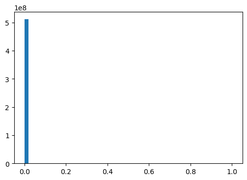

Applying log transform:

log_mut_infos = np.log(mut_infos + eps)

np.isnan(log_mut_infos).sum(), np.isneginf(log_mut_infos).sum(), np.isinf(log_mut_infos).sum()

(0, 0, 0)

CPU times: user 2.35 s, sys: 959 ms, total: 3.31 s
Wall time: 3.3 s

-1.3383214188674972

A little better skewness than before!

hist, bins, _ = plt.hist(log_mut_infos, bins=50,)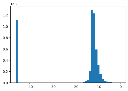

Applying sqrt transform:

sqrt_mut_infos = np.sqrt(mut_infos)

np.isnan(sqrt_mut_infos).sum(), np.isinf(sqrt_mut_infos).sum(), np.isneginf(sqrt_mut_infos).sum()

(0, 0, 0)

CPU times: user 2.38 s, sys: 1.25 s, total: 3.63 s
Wall time: 3.63 s

16.40865608826817

Worse than log transform!

hist, bins, _ = plt.hist(sqrt_mut_infos, bins=50)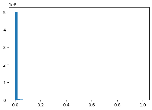

Apply box-cox transfrom:

bcx_mut_infos, *_ = boxcox(mut_infos+eps)

/home/deb/miniconda3/envs/deep/lib/python3.10/site-packages/scipy/stats/_morestats.py:933: RuntimeWarning: overflow encountered in power
  variance = np.var(data**lmb / lmb, axis=0)
/home/deb/miniconda3/envs/deep/lib/python3.10/site-packages/numpy/core/_methods.py:233: RuntimeWarning: invalid value encountered in subtract
  x = asanyarray(arr - arrmean)

np.isnan(bcx_mut_infos).sum(), np.isinf(bcx_mut_infos).sum(), np.isneginf(bcx_mut_infos).sum()

(0, 0, 0)

CPU times: user 2.45 s, sys: 1.04 s, total: 3.49 s
Wall time: 3.49 s

-0.885981418331696

This is the best skew so we’ll go with boxcox.

df_l2r['bcx_mutual_info'] = bcx_mut_infos

hist, bins, _ = plt.hist(bcx_mut_infos, bins=50)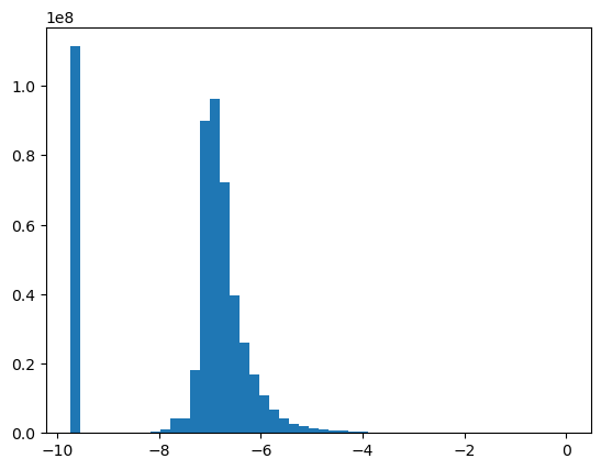

np.min(bcx_mut_infos), np.max(bcx_mut_infos), np.mean(bcx_mut_infos), np.median(bcx_mut_infos)

(-9.734209, -3.6358892e-06, -7.381837, -6.9605794)

# from IPython.display import clear_output

# clear_output(wait=True)

# from tqdm import tqdm
# from time import sleep
# import psutil

# with tqdm(total=100, desc='cpu%', position=1) as cpubar, tqdm(total=100, desc='ram%', position=0) as rambar:
#     while True:
#         rambar.n=psutil.virtual_memory().percent
#         cpubar.n=psutil.cpu_percent()
#         rambar.refresh()
#         cpubar.refresh()
#         sleep(0.5)
#         clear_output(wait=True)

Box plots using matplotlib

fig, (ax1, ax2) = plt.subplots(1, 2, figsize=(12, 5))
ax1 = fig.add_subplot(1, 2, 1)
ax2 = fig.add_subplot(1, 2, 2)

ax1.boxplot(mut_infos, vert=0, notch=True, patch_artist=True)
ax1.set_xscale('log')
ax1.set_xlabel('Mutual Information')

ax2.boxplot(bcx_mut_infos, vert=0, notch=True, patch_artist=True)
# ax2.set_xscale('symlog')
ax2.set_xlabel('Box-Cox Mutual Information')

plt.show()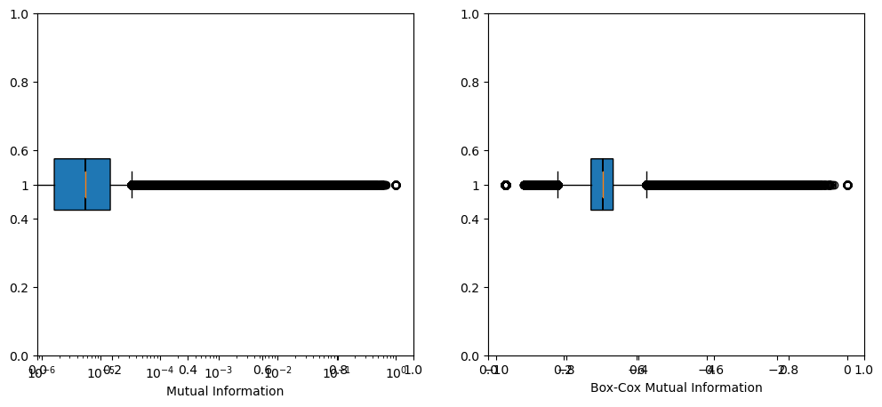

CPU times: user 1min 35s, sys: 9.16 s, total: 1min 44s
Wall time: 1min 44s

Histograms and kde using matplotlib:

fig, (ax1, ax2) = plt.subplots(1, 2, figsize=(12, 5))

# hist, bins, pathches = ax1.hist(df_l2r['mutual_info'])
hist, bins, pathches = ax1.hist(mut_infos)
ax1.set_xlabel('Mutual Information')
ax1.set_ylabel('frequency')
ax1.grid(axis='y', color='black')
ax1.set_yscale('log')

# ax2.hist(df_l2r['bcx_mutual_info'])
ax2.hist(bcx_mut_infos)
ax2.set_xlabel('Boxcox Mutual Information')
ax2.set_ylabel('frequency')
ax2.grid(axis='y', color='black')
ax2.set_yscale('log')

fig.suptitle('Histograms of with and without BoxCox of Mutual Information')
plt.show()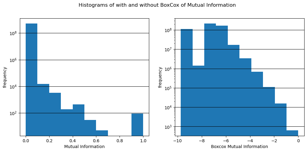

bdrs = [bins[i:i+2] for i in range(0, len(bins)-1)]
pd.DataFrame({'mut_infos bdrs': bdrs, 'counts': hist})

	mut_infos bdrs	counts
0	[0.0, 0.09999963641166687]	511675599.0
1	[0.09999963641166687, 0.19999927282333374]	14848.0
2	[0.19999927282333374, 0.2999989092350006]	3323.0
3	[0.2999989092350006, 0.3999985456466675]	191.0
4	[0.3999985456466675, 0.49999818205833435]	454.0
5	[0.49999818205833435, 0.5999978184700012]	30.0
6	[0.5999978184700012, 0.6999974250793457]	5.0
7	[0.6999974250793457, 0.799997091293335]	0.0
8	[0.799997091293335, 0.8999967575073242]	0.0
9	[0.8999967575073242, 0.9999963641166687]	94.0

# from scipy.stats import gaussian_kde
# density = gaussian_kde(df_l2r['mutual_info'])
# xs = np.linspace(0, 1, 200)
# density.covariance_factor = lambda : .25
# density._compute_covariance()
# plt.plot(xs, density(xs))
# plt.show()

We can now build the Dataloaders object from this dataframe df_collab, by defaultit takes the first column as the user (in our case the token) and the second column as the item (in our case the label), and the third column as the ratings (in our case the frequency):

Build `L2RDataloader`

In this section we’ll build L2RDataLoader for Learning to Rank (L2R)

df_l2r = pd.read_feather(source/'mimic3-9k_tok_lbl.ft')

df_l2r = df_l2r.drop(['mutual_info', 'bcx_mutual_info'], axis=1)
df_l2r.token.nunique(), df_l2r.label.nunique()
df_l2r.head(3)

	label	rank
0	0	866.0
1	1	1022.0
2	2	1156.0

df_tiny: If we need a smaller dataset for quick iterations

Note: For technical reasons behind building a L2RDataloader the number of tokens should be \(x (mod 64) \equiv 8\).

num_toks, num_lbs = 8 + 5*64, 104

# might have to repeat this a few times until the cell asserst true
np.random.seed(101)
rnd_toks = np.random.randint(0, len(df_l2r.token.unique()), size=(num_toks,) )
np.random.seed(101)
rnd_lbs = np.random.randint(0, len(df_l2r.label.unique()), size=(num_lbs,) )
mask = df_l2r.token.isin(rnd_toks) & df_l2r.label.isin(rnd_lbs)
df_tiny = df_l2r[mask].reset_index(drop=True)
test_eq(df_tiny.token.nunique(), num_toks) 
test_eq(df_tiny.label.nunique(), num_lbs) 
# df_tiny.apply(lambda x: x.nunique())

df_tiny.head()

	token	label	rank
0	22	49	1877.0
1	22	239	21308.0
2	22	394	39854.0
3	22	436	8618.0
4	22	561	1646.0

Let’s just delete the df_l2r to free up RAM:

# df_l2r = pd.DataFrame()
# lst = [df_l2r]
# del lst
# del df_l2r
# import gc; gc.collect()

Only for df_tiny:

Due to random sampling the rankings are not uniform i.e., not from 0 to num_toks. A litte preprocessing to make sure that we have uniform rankings for all labels.

grouped = df_tiny.groupby('label', group_keys=False)

def sort_rerank(df, column='rank'):
    df = df.sort_values(by=column)
    df['rank'] = range(len(df))
    return df

df_tiny = grouped.apply(sort_rerank)
dict_grouped = dict(list(df_tiny.groupby('label')))
# checking a random label has ranks 0 thru `num_toks`
a_lbl = random.choice(list(dict_grouped.keys()))
test_eq(range(num_toks), dict_grouped[a_lbl]['rank'].values)

dict_grouped[a_lbl].head()

	token	label	rank
5660	9679	3455	0
8364	13976	3455	1
4620	6801	3455	2
772	1788	3455	3
2748	4458	3455	4

Using Pandas groupby to add quantized relevance scores to each token-label pair based on the corresponding ranks:

grouped = df_tiny.groupby('label')

# dict_grouped = dict(list(grouped))
# _tmp = dict_grouped[16].copy()
# _tmp.head()

def cut(df, qnts, column='rank'):
    num = df.to_numpy()
    bins = np.quantile(num[:, -1], qnts)
    num[:, -1] = len(bins) - np.digitize(num[:, -1], bins)
    # bins = np.quantile(df['rank'], qnts)
    # df[column] = len(bins) - np.digitize(df['rank'], bins)
    # df[column] = pd.qcut(df[column], qnts, labels=labels)
    return num

qnts = np.concatenate([array([0]), np.geomspace(1e-2, 1, 10)])
scored = grouped.apply(cut, qnts)

11.9 ms ± 279 µs per loop (mean ± std. dev. of 15 runs, 50 loops each)

Pandas groupby was just to ellucidate how we do the scoring. It ain’t all that good when dealing with big datasets. So in reality we are going to use tensorized implemnetation. Follow along:

pdl = PreLoadTrans(df_tiny, device=torch.device('cpu'))

If interested please read sourcecode of [PreLoadTrans.quantized_score](https://debjyotiSRoy.github.io/xcube/l2r.data.load.html#preloadtrans.quantized_score):

# %%timeit -n 50 -r 15

scored_toks = pdl.quantized_score()

CPU times: user 1e+03 ns, sys: 0 ns, total: 1e+03 ns
Wall time: 3.34 µs

/home/deb/xcube/xcube/l2r/data/load.py:56: UserWarning: torch.searchsorted(): input value tensor is non-contiguous, this will lower the performance due to extra data copy when converting non-contiguous tensor to contiguous, please use contiguous input value tensor if possible. This message will only appear once per program. (Triggered internally at /opt/conda/conda-bld/pytorch_1670525541990/work/aten/src/ATen/native/BucketizationUtils.h:33.)
  relv_scores = bins.shape[0] - torch.searchsorted(bins.T, data[:, :, -1], right=False) # shape (8922, 57352)

test_eqs(scored_toks.shape, 
         (df_tiny.label.nunique(), df_tiny.token.nunique(), 4), 
         (pdl.num_lbs, pdl.num_toks, 4))

Save if you want to! BTW untar_xxx has got the one for the full dataset:

L(source.glob("**/*scored*.pth"))

(#1) [Path('/home/deb/.xcube/data/mimic3_l2r/scored_tokens.pth')]

Create training and validation split:

Remember: In scored_toks dim 0: labels, dim 1: 4 tuple (token, label, rank, score). Below is an example:

tok, lbl, rank, score = L(scored_toks[97, 32], use_list=True).map(Tensor.item)
ic(tok, lbl, rank, score);

ic| tok: 41514.0, lbl: 8124.0, rank: 234.0, score: 4.0

df_tiny[(df_tiny.token == tok)  & (df_tiny.label == lbl)]

	token	label	rank
23393	41514	8124	234

Remember: For each label the tokens are ranked 0 through num_toks

ranks = scored_toks[:, :, 2].unique(dim=1).sort(-1).values
ranks_shouldbe = torch.arange(scored_toks.shape[1], dtype=torch.float).expand(scored_toks.shape[0], -1)
test_eq(ranks, ranks_shouldbe)

Remember: For each label quantized_score scores the tokens on a log scale based on their ranks. The score scale is 1-101: 101 being the highest score (assigned to most relevant token), and 1 is the lowest score (assigned to least relevant tokens).

scores = scored_toks[:, :, -1].unique(dim=1).sort(-1).values
scores[0]

tensor([  1.,   1.,   1.,   1.,   2.,   2.,   2.,   2.,   2.,   2.,   3.,   3.,
          3.,   3.,   4.,   4.,   4.,   4.,   4.,   4.,   5.,   5.,   5.,   6.,
          6.,   6.,   6.,   6.,   6.,   7.,   7.,   7.,   7.,   7.,   8.,   8.,
          8.,   8.,   8.,   8.,   8.,   8.,   9.,   9.,   9.,   9.,   9.,   9.,
         10.,  10.,  10.,  10.,  11.,  11.,  11.,  11.,  11.,  11.,  12.,  12.,
         12.,  12.,  12.,  13.,  13.,  13.,  13.,  13.,  13.,  14.,  14.,  14.,
         14.,  15.,  15.,  15.,  16.,  16.,  16.,  17.,  17.,  17.,  17.,  17.,
         18.,  18.,  18.,  19.,  19.,  19.,  19.,  20.,  20.,  20.,  20.,  21.,
         21.,  21.,  21.,  22.,  22.,  22.,  22.,  23.,  23.,  23.,  23.,  24.,
         24.,  24.,  25.,  25.,  25.,  26.,  26.,  27.,  27.,  27.,  28.,  28.,
         29.,  29.,  30.,  30.,  31.,  31.,  32.,  32.,  33.,  34.,  34.,  35.,
         36.,  37.,  38.,  39.,  40.,  42.,  43.,  45.,  48.,  51.,  55.,  63.,
        101.])

scored_toks, binned_toks, probs, is_valid, bin_size, bin_bds = pdl.train_val_split()

CPU times: user 90.4 ms, sys: 3.56 ms, total: 94 ms
Wall time: 13.8 ms

val_sl = pdl.pad_split()
test_eq(is_valid.sum(dim=-1).unique().item(), val_sl)
print(f"{val_sl=}")

val_sl=16
CPU times: user 353 ms, sys: 0 ns, total: 353 ms
Wall time: 48.4 ms

Taking a look at the train/valid split for some labels (just to make sure we ticked all boxes!):

df1 = pd.DataFrame(scored_toks[89], columns=['token', 'label', 'rank', 'score']).sort_values(by='score', ascending=False)
df1.head()

	token	label	rank	score
226	28488.0	6820.0	0.0	101.0
225	2274.0	6820.0	1.0	63.0
224	50503.0	6820.0	2.0	55.0
223	56935.0	6820.0	3.0	51.0
222	20945.0	6820.0	4.0	48.0

name = partial(namestr, namespace=globals())
row_vals = apply(torch.Tensor.size, (scored_toks, binned_toks, probs, is_valid, bin_size, bin_bds))
pd.DataFrame(index = list(itertools.chain.from_iterable(apply(name, [scored_toks, binned_toks, probs, is_valid, bin_size, bin_bds]))), columns=['shape'], data={'shape': row_vals})

	shape
scored_toks	(104, 328, 4)
binned_toks	(104, 328)
probs	(104, 328)
is_valid	(104, 328)
bin_size	(11,)
bin_bds	(8, 2)

Lowest numbered bin contains irrelevant tokens for a label, and the highest numbered bin contains most relevant tokens:

df2 = pd.DataFrame({'bin #': range(len(bin_size)), 
                    #'bin_bds': list(bin_bds.numpy()), 
                    'bin_size': bin_size})
df2.head()

	bin #	bin_size
0	0	30
1	1	180
2	2	75
3	3	27
4	4	10

df_toks = pd.read_feather(source/'mimic3-9k_tok.ft')
df_lbs = pd.read_feather(source/'mimic3-9k_lbl.ft')

a_lbl = np.random.choice(pdl.num_lbs)
df_lbs.iloc[[a_lbl]]
# df_lbs.loc[[a_lbl]]

	lbl	lbl_val
52	52	018.95

df3 = pd.DataFrame({'token': scored_toks[a_lbl, :, 0] ,'score': scored_toks[a_lbl, :, -1], 'probs': probs[a_lbl], 
                    'binned_toks': binned_toks[a_lbl], 
                    #'bds': list(bin_bds[binned_toks[a_lbl]].numpy()), 
                    'size': bin_size[binned_toks[a_lbl]], 
                    'is_valid': is_valid[a_lbl]})
df3 = df_toks.merge(df3, on='token')
df3.sort_values(by='score', ascending=False).head(20)

	token	tok_val	score	probs	binned_toks	size	is_valid
30	4924	distance	101.0	0.333333	10	1	0.0
25	4056	defined	63.0	0.333333	6	1	1.0
10	2100	wnl	55.0	0.166667	5	4	0.0
2	436	change	51.0	0.166667	5	4	0.0
3	591	motion	48.0	0.166667	5	4	0.0
5	1327	residual	45.0	0.166667	5	4	0.0
0	22	patient	43.0	0.066667	4	10	0.0
7	1788	thursday	42.0	0.066667	4	10	0.0
6	1699	clopidogrel	40.0	0.066667	4	10	0.0
9	2021	saturations	39.0	0.066667	4	10	0.0
8	1944	4l	38.0	0.066667	4	10	0.0
11	2265	hemodynamics	37.0	0.066667	4	10	0.0
13	2467	according	36.0	0.066667	4	10	0.0
12	2274	medial	35.0	0.066667	4	10	0.0
14	2998	synagis	34.0	0.066667	4	10	1.0
15	3159	film	34.0	0.066667	4	10	0.0
20	3748	dispo	33.0	0.024691	3	27	0.0
16	3401	twenty	32.0	0.024691	3	27	0.0
18	3575	attached	32.0	0.024691	3	27	0.0
27	4598	stopping	31.0	0.024691	3	27	0.0

test_eqs(is_valid[a_lbl].sum(), df3['is_valid'].sum(), pdl.val_sl)

df3[df3['is_valid'] == 1].sort_values(by='score', ascending=False)#.groupby('binned_toks').size()

	token	tok_val	score	probs	binned_toks	size	is_valid
25	4056	defined	63.0	0.333333	6	1	1.0
14	2998	synagis	34.0	0.066667	4	10	1.0
29	4750	ccy	29.0	0.024691	3	27	1.0
17	3469	brace	28.0	0.024691	3	27	1.0
28	4608	pericarditis	25.0	0.024691	3	27	1.0
170	32817	cadmium	19.0	0.008889	2	75	1.0
195	36874	discrepant	18.0	0.008889	2	75	1.0
47	8157	fundi	17.0	0.008889	2	75	1.0
272	48514	vorinostat	13.0	0.008889	2	75	1.0
306	54261	entroclysis	13.0	0.008889	2	75	1.0
114	21311	icbg	8.0	0.003704	1	180	1.0
183	35391	bender	5.0	0.003704	1	180	1.0
216	39783	susbsequently	4.0	0.003704	1	180	1.0
261	46217	cuurently	3.0	0.003704	1	180	1.0
302	53619	transfred	1.0	0.022222	0	30	1.0
322	56325	psuedoanuerysm	1.0	0.022222	0	30	1.0

top_lens = pdl.count_topbins()
test_eq(top_lens.shape, [pdl.num_lbs])
print(f"For {torch.where(top_lens >= 1)[0].numel()} labels out of total {pdl.num_lbs}, in the validation set we have at least one top 2 bin")

For 56 labels out of total 104, in the validation set we have at least one top 2 bin

Prepare the train/val dataset:

trn_dset, val_dset = pdl.datasets()

test_eq(val_dset.shape, (scored_toks.shape[0], val_sl, scored_toks.shape[2]))
test_eq(trn_dset.shape, scored_toks.shape) 
ic(trn_dset.shape, val_dset.shape);

ic| trn_dset.shape: torch.Size([104, 328, 4])
    val_dset.shape: torch.Size([104, 16, 4])

Again, untar_xxx has got the trn/val split for the full dataset:

L(source.glob("**/*split*.pkl"))

(#1) [Path('/home/deb/.xcube/data/mimic3_l2r/trn_val_split.pkl')]

If you want to load the splits for the full dataset:

trn_dset, val_dset = torch.load(source/'trn_val_split.pkl')
ic(trn_dset.shape, val_dset.shape);

ic| trn_dset.shape: torch.Size([8922, 57352, 4])
    val_dset.shape: torch.Size([8922, 32, 4])

Now we are ready to create the train/valid DataLoaders:

Implementation note: We have written the training dataloader which we call L2RDataLoader. It ofcourse inherits from fastai’s incredibly hackable DataLoader class. In a little more technical terms, another way to say this is that L2RDataLoader provides different implementation of the callbacks before_iter and create_batches. However for the validation dataloader we directly use fastai’s DataLoader. Lastly, we store the training and validation dataloder objects using fastai’s DataLoaders class.

bs_full = 32
bs_tiny = 8
sl = 64
lbs_chunks_full = 4
lbs_chunks_tiny = 32
trn_dl = L2RDataLoader(dataset=trn_dset, sl=sl, bs=bs_tiny, lbs_chunks=lbs_chunks_tiny, shuffle=False, after_batch=partial(to_device, device=default_device(use=True)), num_workers=0)

Don’t forget to check the length

len(trn_dl)

ic(trn_dl.num_workers, trn_dl.fake_l.num_workers);

ic| trn_dl.num_workers: 1, trn_dl.fake_l.num_workers: 0

xb = trn_dl.one_batch()
ic(xb.shape, xb.device);

ic| xb.shape: torch.Size([8, 4, 64, 4])
    xb.device: device(type='cuda', index=0)

A fake rundown of the training loop to make sure the training dataloader got created alright:

for xb in progress_bar(trn_dl):
    time.sleep(0.01)

100.00% [24/24 00:00<00:00]

CPU times: user 1.4 s, sys: 12.8 ms, total: 1.41 s
Wall time: 298 ms

from fastai.data.load import DataLoader
from fastai.data.core import DataLoaders

val_dset = val_dset.unsqueeze(0)
val_dl = DataLoader(val_dset, bs=1, shuffle=False, after_batch=partial(to_device, device=default_device()), num_workers=0)
ic(val_dl.num_workers, val_dl.fake_l.num_workers);

ic| val_dl.num_workers: 1, val_dl.fake_l.num_workers: 0

xb = val_dl.one_batch()
ic(xb.shape, xb.device);

ic| xb.shape: torch.Size([1, 104, 16, 4])
    xb.device: device(type='cuda', index=0)

A fake rundown of the validation set to make sure the validation dataloader got created alright:

for xb in progress_bar(val_dl):
    time.sleep(0.01)

100.00% [1/1 00:00<00:00]

CPU times: user 6.07 ms, sys: 0 ns, total: 6.07 ms
Wall time: 15.8 ms

Bunching together the training and validation dataloaders:

dls = DataLoaders(trn_dl, val_dl)

Training

…yes, finally!

Keeping records:

m = ['lin', 'nn']
algos = ['ranknet', 'lambdarank']
idx = pd.Index(['tiny', 'full'], name='dataset')
cols = pd.MultiIndex.from_product([m, algos], names = ['model', 'algo'])

df = pd.DataFrame(columns=cols, index=idx)
df[:] = 'TBD'

df.loc['tiny']['nn']['ranknet'] = "{'grad_func': functools.partial(<function rank_loss3 at 0x7f6f87e800d0>, gain_fn='exp', k=6), 'opt_func': functools.partial(<function RMSProp at 0x7f6f87e31870>, mom=0.9, wd=0.2), 'opt': None, 'lr': 0.001, 'loss_func': <function loss_fn2 at 0x7f6f7cdb1990>, 'num_factors': 200, 'n_act': 100, 'num_lbs': 105, 'num_toks': 329, 'seed': 877979, 'epochs': 15, 'best': 75.66}"
df.loc['tiny']['lin']['ranknet'] = "{'grad_func': functools.partial(<function rank_loss3 at 0x7f6f87e800d0>, gain_fn='exp', k=6), 'opt_func': functools.partial(<function SGD at 0x7f6f87e31750>, mom=0.9), 'opt': None, 'lr': 0.0001, 'loss_func': <function loss_fn2 at 0x7f6f73f748b0>, 'num_factors': 200, 'num_lbs': 105, 'num_toks': 329, 'seed': 877979, 'epochs': 15, 'best': 75}"
df.loc['tiny']['nn']['lambdarank'] = "{'grad_func': functools.partial(<function rank_loss3 at 0x7fdc0ed6ad40>, gain_fn='exp', k=15, lambrank=True), 'opt_func': functools.partial(<function RMSProp at 0x7fdc0ed28280>, mom=0.9, wd=0.0), 'opt': <fastai.optimizer.Optimizer object at 0x7fdc0ede79a0>, 'lr': 0.001, 'loss_func': <function loss_fn2 at 0x7fdc0ed6ae60>, 'lr_max': 0.01445439737290144, 'num_factors': 200, 'n_act': 100, 'num_lbs': 105, 'num_toks': 329, 'seed': 1, 'epochs': 15, 'best': 'ndcg_at_6 = 39.05', 'model': 'L2R_NN(\\n  (token_factors): Embedding(329, 200, padding_idx=328)\\n  (label_factors): Embedding(105, 200, padding_idx=104)\\n  (layers): Sequential(\\n    (0): Linear(in_features=200, out_features=100, bias=True)\\n    (1): ReLU()\\n    (2): Linear(in_features=100, out_features=1, bias=True)\\n    (3): Dropout(p=0.2, inplace=False)\\n  )\\n)\\n self.n_act = 100, self.dp = 0.2'}"
df.loc['tiny']['lin']['lambdarank'] = "{'grad_func': functools.partial(<function rank_loss3 at 0x7f4c7dd42c20>, gain_fn='exp', k=15, lambrank=True), 'opt_func': functools.partial(<function RMSProp at 0x7f4c7dd04160>, mom=0.9, wd=0.0), 'opt': <fastai.optimizer.Optimizer object at 0x7f4c5c1da410>, 'lr': 0.007, 'loss_func': <function loss_fn2 at 0x7f4c74b9add0>, 'num_factors': 200, 'n_act': None, 'num_lbs': 105, 'num_toks': 329, 'seed': 1, 'epochs': 15, 'best': 52.21}"

df.loc['full']['nn']['ranknet'] = 'TBD'
df.loc['full']['lin']['ranknet'] = {'lr': 1e-5, 'opt': 'partial(SGD, mom=0.9, wd=0.0)', 'best': 63.73, 'epochs': 3, 'seed': 1, 'gain': 'cubic', 'factors': 100}
df.loc['full']['nn']['lambdarank'] = 'TBD'
df.loc['full']['lin']['lambdarank'] = {'lr': [7e-4, 7e-4, 7e-4], 'opt': 'partial(RMSProp, mom=0.9, wd=0.0)', 'best': 12.85, 'epochs': [4, 2, 4, 4], 'seed': 1, 'gain': 'exp', 'factors': 200}

df

model	lin		nn
algo	ranknet	lambdarank	ranknet	lambdarank
dataset
tiny	{'grad_func': functools.partial(<function rank_loss3 at 0x7f6f87e800d0>, gain_fn='exp', k=6), 'opt_func': functools.partial(<function SGD at 0x7f6f87e31750>, mom=0.9), 'opt': None, 'lr': 0.0001, 'loss_func': <function loss_fn2 at 0x7f6f73f748b0>, 'num_factors': 200, 'num_lbs': 105, 'num_toks': 329, 'seed': 877979, 'epochs': 15, 'best': 75}	{'grad_func': functools.partial(<function rank_loss3 at 0x7f4c7dd42c20>, gain_fn='exp', k=15, lambrank=True), 'opt_func': functools.partial(<function RMSProp at 0x7f4c7dd04160>, mom=0.9, wd=0.0), 'opt': <fastai.optimizer.Optimizer object at 0x7f4c5c1da410>, 'lr': 0.007, 'loss_func': <function loss_fn2 at 0x7f4c74b9add0>, 'num_factors': 200, 'n_act': None, 'num_lbs': 105, 'num_toks': 329, 'seed': 1, 'epochs': 15, 'best': 52.21}	{'grad_func': functools.partial(<function rank_loss3 at 0x7f6f87e800d0>, gain_fn='exp', k=6), 'opt_func': functools.partial(<function RMSProp at 0x7f6f87e31870>, mom=0.9, wd=0.2), 'opt': None, 'lr': 0.001, 'loss_func': <function loss_fn2 at 0x7f6f7cdb1990>, 'num_factors': 200, 'n_act': 100, 'num_lbs': 105, 'num_toks': 329, 'seed': 877979, 'epochs': 15, 'best': 75.66}	{'grad_func': functools.partial(<function rank_loss3 at 0x7fdc0ed6ad40>, gain_fn='exp', k=15, lambrank=True), 'opt_func': functools.partial(<function RMSProp at 0x7fdc0ed28280>, mom=0.9, wd=0.0), 'opt': <fastai.optimizer.Optimizer object at 0x7fdc0ede79a0>, 'lr': 0.001, 'loss_func': <function loss_fn2 at 0x7fdc0ed6ae60>, 'lr_max': 0.01445439737290144, 'num_factors': 200, 'n_act': 100, 'num_lbs': 105, 'num_toks': 329, 'seed': 1, 'epochs': 15, 'best': 'ndcg_at_6 = 39.05', 'model': 'L2R_NN(\n (token_factors): Embedding(329, 200, padding_idx=328)\n (label_factors): Embedding(105, 200, paddin...
full	{'lr': 1e-05, 'opt': 'partial(SGD, mom=0.9, wd=0.0)', 'best': 63.73, 'epochs': 3, 'seed': 1, 'gain': 'cubic', 'factors': 100}	{'lr': [0.0007, 0.0007, 0.0007], 'opt': 'partial(RMSProp, mom=0.9, wd=0.0)', 'best': 12.85, 'epochs': [4, 2, 4, 4], 'seed': 1, 'gain': 'exp', 'factors': 200}	TBD	TBD

Get the `DataLoaders`:

tmp = Path.cwd()/'tmp'
tmp.mkdir(exist_ok=True)
list_files(str(tmp))

tmp/
    mimic3-9k_dls_clas_tiny.pkl
    nn_lambdarank_tiny.pth
    mimic3-9k_dls_clas_tiny_r.pkl
    dls_full.pkl
    dls_tiny.pkl
    lin_lambdarank_full.pth
    lin_lambdarank_tiny.pth
    .ipynb_checkpoints/
    models/
        mimic3-9k_lm_finetuned_r.pth
        mimic3-9k_clas_full.pth
        mimic3-9k_clas_tiny_r.pth
        mimic3-9k_lm_finetuned.pth
        mimic3-9k_clas_tiny_vocab.pkl
        mimic3-9k_clas_tiny_r_vocab.pkl
        mimic3-9k_clas_tiny.pth
        mimic3-9k_clas_full_vocab.pkl

set_seed(1, True)

Setting the fname capturing which model (neural net vs linear) we want to run, which algorithm (ranknet vs lambdarank) and on which dataset (tiny vs full). This fname is then used to automaticall grab the appropriate dataloder, make the model and set relevant learner parameters.

fname = 'lin_lambdarank_tiny'
monitor = 'ndcg_at_6' if 'lambda' in fname else 'acc'
s = fname.split('_')
print(f'We will run a {s[0]} model using the {s[1]} algorithm on the {s[2]} dataset. And our metric of interest(moi) is {monitor}.')

We will run a lin model using the lambdarank algorithm on the tiny dataset. And our metric of interest(moi) is ndcg_at_6.

CPU times: user 11.7 ms, sys: 8.62 s, total: 8.63 s
Wall time: 15.3 s

Make the Model:

Based on the dataset:

Datasizes = namedtuple("Datasizes", ('num_lbs', 'num_toks', 'num_factors'))
sizes = Datasizes(*dls.dataset.shape[:-1], 200) # or pdl.num_lbs, pdl.num_toks, 200
sizes

Datasizes(num_lbs=104, num_toks=328, num_factors=200)

model = (L2R_NN(*sizes, layers=[100], embed_p=0.2, ps=[0.1], bn_final=False, y_range=None) if 'nn' in fname else L2R_DotProductBias(*sizes,y_range=None)).to(default_device())

Create the Learner and train:

from fastai.optimizer import *

def grab_learner_params(fname):
    "Get relevant `learner` params depending on the `fname`"
    
    nn, lambrank, tiny =  [sp == n for sp, n in zip(fname.split('_'), ['nn', 'lambdarank', 'tiny'])]
    # create a dictionary that maps binary conditions to tuple (nn, lambdarank, tiny)
    conditions = {
        (True, True, True):  dict(lr = 1e-3, lambrank = lambrank, opt_func = partial(RMSProp, mom=0.9, wd=0.0)),   # nn_lambdarank_tiny
        (True, True, False): dict(lr = 1e-2, lambrank = lambrank, opt_func = partial(Adam, mom=0.9, wd=0.1)),   # nn_lambdarank_full
        (True, False, True):  dict(lr = 1e-2, lambrank = lambrank, opt_func = partial(RMSProp, mom=0.9, wd=0.2)),  # nn_ranknet_tiny
        (True, False, False): dict(lr = None, lambrank = lambrank, opt_func = None),  # nn_ranknet_full
        (False, True, True): dict(lr = 7e-3, lambrank = lambrank, opt_func = partial(RMSProp, mom=0.9, wd=0.0)),   # lin_lambdarank_tiny
        (False, True, False): dict(lr = 7e-3, lambrank = lambrank, opt_func = partial(RMSProp, mom=0.9, wd=0.0)),  # lin_lambdarank_full
        (False, False, True): dict(lr = 1e-4, lambrank = lambrank, opt_func = None),  # lin_ranknet_tiny
        (False, False, False): dict(lr = None, lambrank = lambrank, opt_func = None), # lin_ranknet_full
    }
    learner_params = conditions.get((nn, lambrank, tiny), (True, True, True))
    default_cbs = [TrainEval(), TrackResults(train_metrics=False, beta=0.98), ProgressBarCallback(), Monitor(), SaveCallBack(fname, monitor=monitor)]
    grad_fn = partial(rank_loss3, gain_fn='exp', k=15)
    learner_params = {**learner_params, **{'cbs':default_cbs, 'grad_fn':grad_fn}}
    return learner_params

learner_params = grab_learner_params(fname)
learner_params

{'lr': 0.007,
 'lambrank': True,
 'opt_func': functools.partial(<function RMSProp>, mom=0.9, wd=0.0),
 'cbs': [TrainEval, TrackResults, ProgressBarCallback, Monitor, SaveCallBack],
 'grad_fn': functools.partial(<function rank_loss3>, gain_fn='exp', k=15)}

learner = get_learner(model, dls, **learner_params)

learner.path = tmp

Let’s record some useful hyperparameters in a record dict which we can store in the dataframe in the record keeping section:

learner_attrs = ['grad_func', 'opt_func', 'opt', 'lr', 'loss_func', 'lr_max']
model_attrs = ['num_factors', 'n_act', 'num_lbs', 'num_toks']
record = dict(zip(learner_attrs + model_attrs, getattrs(learner, *learner_attrs) + getattrs(learner.model, *model_attrs)))
record['seed'] = torch.initial_seed()
record['epochs'] = 15
record['best'] = f'{monitor} = 37.97'
record['model'] = str(learner.model)
str(record)

"{'grad_func': functools.partial(<function rank_loss3>, gain_fn='exp', k=15, lambrank=True), 'opt_func': functools.partial(<function RMSProp>, mom=0.9, wd=0.0), 'opt': None, 'lr': 0.007, 'loss_func': <function loss_fn2>, 'lr_max': None, 'num_factors': 200, 'n_act': None, 'num_lbs': 105, 'num_toks': 329, 'seed': 1, 'epochs': 15, 'best': 'ndcg_at_6 = 37.97', 'model': 'L2R_DotProductBias(\\n  (token_factors): Embedding(329, 200, padding_idx=328)\\n  (token_bias): Embedding(329, 1, padding_idx=328)\\n  (label_factors): Embedding(105, 200, padding_idx=104)\\n  (label_bias): Embedding(105, 1, padding_idx=104)\\n)'}"

Finding learning rate:

from fastai.callback.schedule import valley, slide, steep

learner.xrl_find(num_it=300, suggest_funcs=(valley, slide, steep))

Smoothing ndcg_at_6
0 True 1.2428 0.732 0.6955 0.6977
0 False NA NA NA NA
1 True 1.2239 0.7202 0.6793 0.6992
1 False NA NA NA NA

SuggestedLRs(valley=0.010964781977236271, slide=0.05248074606060982, steep=0.07356422394514084)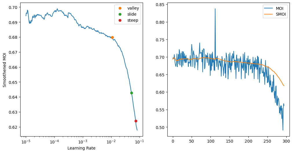

# learner.fit_one_cycle(1, lr_max=0.014454)
# learner.fit_one_cycle(15, lr_max=0.014454)
# learner.fit_one_cycle(1, lr_max=0.0611)
# learner.fit_one_cycle(3, lr_max=0.0611)
# learner.fit_one_cycle(1, lr_max=0.01239)
# learner.fit_one_cycle(3, lr_max=0.01239)
learner.fit_one_cycle(1, lr_max=0.010964)
learner.fit_one_cycle(3, lr_max=0.010964)

0 True 1.3046 NA NA NA
0 False 0.9848 0.774 0.7596 0.7612
0 True 1.2438 NA NA NA
0 False 0.9702 0.7635 0.7474 0.7637
1 True 1.2317 NA NA NA
1 False 0.9498 0.7723 0.7571 0.7631
2 True 1.2137 NA NA NA
2 False 0.9418 0.7711 0.756 0.764

learner.track_results.plot_sched()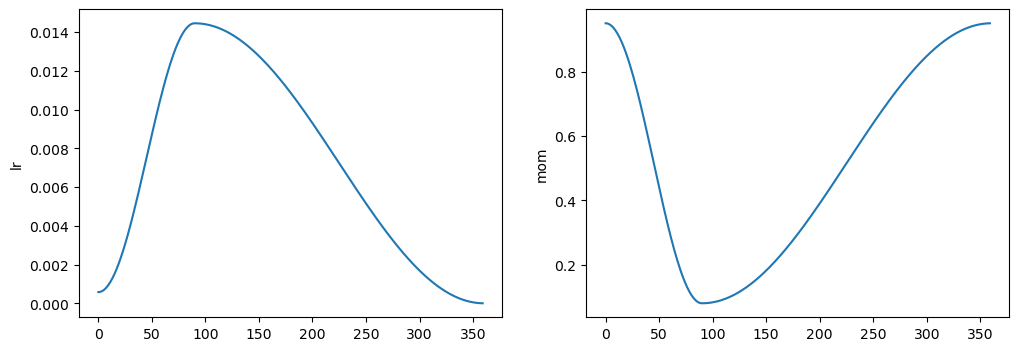

# len(learner.cbs[1].grads_full['token_factors.weight'])
# learner.cbs
# learner.track_results
# learner.opt.hypers[-1]

learner = learner.load(fname, device=default_device())

learner.validate()

0 False 1.0591 0.7812 0.7686 0.76

learner.cbs[-1].best = 0.7686

# emb_szs = get_emb_sz(dls.train_ds, {})

Plots

Plotting losses and metrics:

fig, axes = plt.subplots(2, 2, figsize=(15,8))
loss = L(loss_logger).map(torch.Tensor.item)
val_loss = L(metric_logger).itemgot(0)
val_acc = L(metric_logger).itemgot(-1)
val_ndcg = L(metric_logger).itemgot(2)

# axes[0,0].scatter(range(len(loss)), loss)
axes[0,0].plot(range(len(loss)), loss)
axes[0,0].set_xlabel('batches*epochs')
axes[0,0].set_ylabel('train loss')

axes[0,1].plot(val_loss)
axes[0,1].set_xlabel('epochs')
axes[0,1].set_ylabel('val loss')

axes[1, 0].plot(val_acc)
axes[1,0].set_xlabel('epochs')
axes[1,0].set_ylabel('val accuracy')

axes[1,1].plot(val_ndcg)
axes[1,1].set_xlabel('epochs')
axes[1,1].set_ylabel('val ndcg@6 (candidate 16)')

plt.show()

Plotting Statistics of the Model Parameters

fig, axes = plt.subplots(2,2, figsize=(15,8), sharex=True)
for (k,v), ax in zip(grad_logger.items(), axes.flatten()):
    mean_grads = L(v).map(compose(torch.Tensor.square, torch.Tensor.mean, torch.Tensor.sqrt, torch.Tensor.item))
    # sparsity = L(v).map(sparsity)
    ax.plot(mean_grads, color='r', label='mean')
    ax.set_ylabel(k)
    # ax_a = ax.twinx()
    # ax_a.plot(sparsity, color='b', label='sparsity')
    ax.legend(loc='best')
    # ax_a.legend(loc='best')
fig.suptitle('RMS of the Gradients of Model Parameters')
plt.show()

def sparsity(t): 
    return 1 - (torch.count_nonzero(t)/t.numel()).item()

fig, axes = plt.subplots(2,2, figsize=(15,8), sharex=True)
for (k,v), ax in zip(grad_logger.items(), axes.flatten()):
    sp = L(v).map(sparsity)
    ax.scatter(range(len(sp)), sp, color='r', label='sparsity')
    ax.set_ylabel(k)
    # ax_a = ax.twinx()
    # ax_a.plot(sparsity, color='b', label='sparsity')
    ax.legend(loc='best')
    # ax_a.legend(loc='best')
fig.suptitle('Sparsity of the Model Parameters')
plt.show()

Analysis to find out what the L2R model is upto:

dataset = to_device(learner.dls.train.dataset)

_ndcg_at_k = ndcg_at_k(dataset, learner.model, k=15)

CPU times: user 5.73 s, sys: 0 ns, total: 5.73 s
Wall time: 5.86 s

ic(_ndcg_at_k.shape, _ndcg_at_k.min(), _ndcg_at_k.mean(), _ndcg_at_k.max(), _ndcg_at_k.median(), _ndcg_at_k.std());

ic| _ndcg_at_k.shape: torch.Size([1, 8922])
    _ndcg_at_k.min(): tensor(4.0372e-19, device='cuda:0')
    _ndcg_at_k.mean(): tensor(0.3494, device='cuda:0')
    _ndcg_at_k.max(): tensor(0.9934, device='cuda:0')
    _ndcg_at_k.median(): tensor(0.3283, device='cuda:0')
    _ndcg_at_k.std(): tensor(0.2672, device='cuda:0')

qnts = torch.linspace(0, 1, 100)
plt.plot(qnts, _ndcg_at_k.cpu().quantile(qnts, dim=-1).view(-1));
plt.xlabel('quantiles')
plt.ylabel('ndcg@k')
plt.title('Quantile Plot for ndcg@k of all the labels')
plt.show()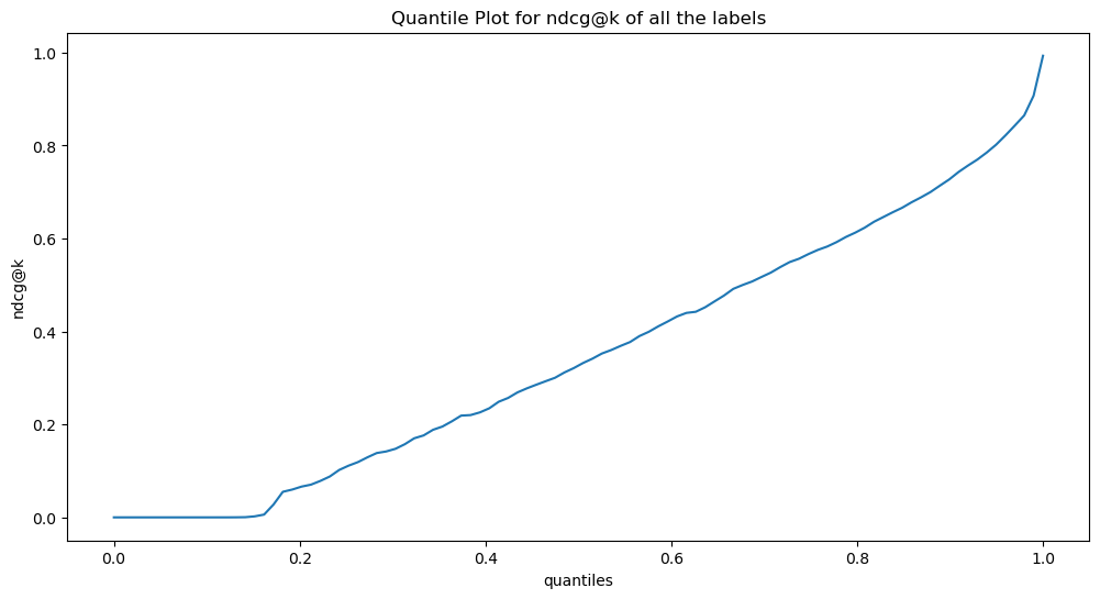

acc = accuracy(dataset, learner.model)

CPU times: user 276 ms, sys: 0 ns, total: 276 ms
Wall time: 286 ms

ic(acc.shape, acc.min(), acc.mean(), acc.max(), acc.median(), acc.std());

ic| acc.shape: torch.Size([1, 104])
    acc.min(): tensor(0.6281, device='cuda:0')
    acc.mean(): tensor(0.7566, device='cuda:0')
    acc.max(): tensor(0.7964, device='cuda:0')
    acc.median(): tensor(0.7626, device='cuda:0')
    acc.std(): tensor(0.0296, device='cuda:0')

Let’s pick some random labels and see the rankings produced by the model:

df_res, df_ndcg= learner.show_results(k=15)

df_ndcg[df_ndcg.ndcg_at_k >= 0.5]

	labels	ndcg_at_k
5	5644	0.505686
6	5102	0.608648
8	1804	0.594066
11	2355	0.581916
22	8161	0.500200
28	2877	0.557069
30	129	0.706364
33	1245	0.733052
35	16	0.618285
38	1208	0.518697
53	6305	0.767246
58	1068	0.748479
89	1104	0.534632
91	5173	0.572957
92	934	0.650478

df_ndcg.head(10)

	labels	ndcg_at_k
0	8526	4.967139e-16
1	7962	4.525589e-15
2	3987	5.901048e-01
3	6165	2.050589e-13
4	6168	3.538292e-10
5	2640	3.429065e-13
6	862	1.326269e-14
7	2750	2.974324e-14
8	7083	1.927360e-12
9	7382	3.322057e-13

df_res

label	4565						6569				...	1047				1349
key2	tok	lbl	rank	score	preds	model_rank	tok	lbl	rank	score	...	rank	score	preds	model_rank	tok	lbl	rank	score	preds	model_rank
toks
0	51577.0	4565.0	53188.0	1.0	-41.782745	54696.0	51577.0	6569.0	51079.0	2.0	...	50834.0	2.0	-45.150726	55395.0	51577.0	1349.0	53188.0	1.0	-32.015938	34146.0
1	52360.0	4565.0	36926.0	5.0	-36.372681	46839.0	52360.0	6569.0	35079.0	6.0	...	21593.0	11.0	-37.832306	46060.0	52360.0	1349.0	36928.0	5.0	-38.207287	48127.0
2	37101.0	4565.0	23703.0	10.0	-42.323380	55161.0	37101.0	6569.0	40328.0	4.0	...	32080.0	7.0	-31.006001	31124.0	37101.0	1349.0	23697.0	10.0	-38.562450	48761.0
3	37705.0	4565.0	24090.0	10.0	-24.040859	17313.0	37705.0	6569.0	40714.0	4.0	...	32466.0	7.0	-29.984770	28882.0	37705.0	1349.0	24084.0	10.0	-35.929695	43524.0
4	14257.0	4565.0	4641.0	28.0	-27.471664	24536.0	14257.0	6569.0	13676.0	16.0	...	12842.0	17.0	-24.753557	18343.0	14257.0	1349.0	4612.0	28.0	-25.678783	19302.0
...	...	...	...	...	...	...	...	...	...	...	...	...	...	...	...	...	...	...	...	...	...
57347	4537.0	4565.0	16797.0	14.0	-17.453377	7259.0	4537.0	6569.0	3001.0	32.0	...	3601.0	30.0	-15.355591	2176.0	4537.0	1349.0	16785.0	14.0	-18.952923	8060.0
57348	1622.0	4565.0	1927.0	37.0	-14.181708	4227.0	1622.0	6569.0	33860.0	6.0	...	950.0	45.0	-9.783297	112.0	1622.0	1349.0	1878.0	37.0	-18.222450	7188.0
57349	16373.0	4565.0	5797.0	25.0	-19.083836	9199.0	16373.0	6569.0	15122.0	15.0	...	16773.0	14.0	-17.529833	5061.0	16373.0	1349.0	5781.0	25.0	-29.995731	29059.0
57350	43863.0	4565.0	31410.0	7.0	-39.971527	52866.0	43863.0	6569.0	25107.0	9.0	...	40880.0	4.0	-26.384148	21487.0	43863.0	1349.0	31405.0	7.0	-34.167110	39351.0
57351	11619.0	4565.0	5573.0	26.0	-26.214912	21706.0	11619.0	6569.0	14697.0	15.0	...	16236.0	14.0	-22.856853	14855.0	11619.0	1349.0	5553.0	26.0	-25.605606	19152.0

57352 rows × 600 columns

df_lbl = df_res.loc[:, 934]
df_lbl

key2	tok	lbl	rank	score	preds	model_rank
toks
0	51577.0	934.0	53188.0	1.0	-19.667917	5888.0
1	52360.0	934.0	34324.0	6.0	-31.594564	32015.0
2	37101.0	934.0	31239.0	7.0	-39.322235	50443.0
3	37705.0	934.0	31626.0	7.0	-41.059654	52976.0
4	14257.0	934.0	12569.0	17.0	-24.408052	15270.0
...	...	...	...	...	...	...
57347	4537.0	934.0	3247.0	31.0	-17.787853	3021.0
57348	1622.0	934.0	9534.0	20.0	-17.016525	2166.0
57349	16373.0	934.0	14253.0	15.0	-25.219761	16950.0
57350	43863.0	934.0	43040.0	4.0	-41.898140	53898.0
57351	11619.0	934.0	13718.0	16.0	-31.796059	32533.0

57352 rows × 6 columns

df2 = df_lbl.sort_values(by='rank').head(15)
df2

key2	tok	lbl	rank	score	preds	model_rank
toks
38712	9429.0	934.0	0.0	101.0	2.399450	1.0
30106	31007.0	934.0	1.0	100.0	-5.644907	17.0
50302	5150.0	934.0	2.0	100.0	-0.324139	3.0
20514	42988.0	934.0	3.0	100.0	-5.003191	13.0
16688	48423.0	934.0	4.0	100.0	5.765238	0.0
39796	21173.0	934.0	5.0	100.0	-10.666720	136.0
26300	24115.0	934.0	6.0	99.0	-7.009228	26.0
29622	24101.0	934.0	7.0	97.0	-11.829512	220.0
29563	52417.0	934.0	8.0	96.0	-6.944853	25.0
20455	52706.0	934.0	9.0	95.0	-4.231724	11.0
40045	56483.0	934.0	10.0	94.0	-8.524904	49.0
39812	12054.0	934.0	11.0	92.0	-8.043360	38.0
1172	40229.0	934.0	12.0	92.0	-13.823061	541.0
13627	41785.0	934.0	13.0	91.0	-14.363610	696.0
56275	47498.0	934.0	14.0	90.0	-10.826721	151.0

# idcg_at_k = pow(2, df2['score']) * (1 / np.log2(df2['rank']+2)  )
# idcg_at_k

# df3 = df_lbl.sort_values(by='model_rank').head(10)
# df3

# dcg_at_k = pow(2, df3['score'])  *(1/np.log2(df3['model_rank']+2))
# dcg_at_k

# dcg_at_k.sum()/idcg_at_k.sum()